In this tutorial and analysis, we’ll apply topic modelling to Danish Trustpilot reviews of “3” (“three” in other countries), my current telecommunications provider. I’m dissatisfied with their customer service and thought this would be an interesting use case for topic modelling. With this approach, we can try to find out which aspects of the customer experience come up in positive and negative reviews.
I used a Python script to scrape 4000 customer reviews of “3” from trustpilot.dk between January 2015 and October 2017.
For more details on topic modelling with the tidytext package by Julia Silge and David Robinson, check out their book.
Required packages
if(!require("pacman")) install.packages("pacman")
pacman::p_load(tidyverse,tidytext,tm,topicmodels,magrittr,
               jtools,gridExtra,knitr,widyr,ggraph,igraph,kableExtra)

if(!require("devtools")) install.packages("devtools")
devtools::install_github("56north/happyorsad")
library(happyorsad)
Customising a ggplot theme
Improving the look of figures in ggplot2 is fairly simple. For consistency, we’ll create a clean and simple theme based on the APA theme from the jtools package and change some of the features. The background colour will be set to a light grey hue. The grid lines are omitted in the APA theme.
my_theme <- function() {
  theme_apa(legend.pos   = "none") +
  theme(panel.background = element_rect(fill = "gray96", colour = "gray96"),
        plot.background  = element_rect(fill = "gray96", colour = "gray96"),
        plot.margin      = margin(1, 1, 1, 1, "cm"),
        panel.border     = element_blank(),        # facet border
        strip.background = element_blank())        # facet title background
}
Loading and preparing the data
Our data frame has two columns: a variable called Name containing the name of the reviewer/author, which will function as a variable to identify each documen; a variable called Review containing individual reviews.
df <- read_csv2("https://raw.githubusercontent.com/PeerChristensen/trustpilot_reviews/master/3reviewsB.csv")

df %<>%
  select(-X1) %>%                                            # remove unnecessary column
  filter(Name != "John M. Sebastian")                        # remove one very odd review
Given that our reviews are in Danish, we can use the happyorsad package to compute a sentiment score for each review. Scores are based on a Danish list of sentiment words and scores put together by Finn Årup Nielsen. We will also make sure that all words are in lowercase, and remove a bunch of pre-defined Danish stop words and frequent verbs.
df %<>%
  mutate(Sentiment = map_int(df$Review,happyorsad,"da")) %>%
  mutate(Review = tolower(Review)) %>%
  mutate(Review = removeWords(Review, c("så", "3", "kan","få","får","fik", stopwords("danish"))))
Distribution of sentiment scores
In the density plot below, we see how sentiment scores are distributed with a median score of 2. As you can probably tell, we’re dealing with a fairly mediocre provider. However, we still want to know why the company has a 6.7 rating out of 10.
In a very crude way, we can put positive and negative reviews in separate data frames and perform topic modelling on each in order to explore what reviewers like and dislike about 3.
df %>%
  ggplot(aes(x = Sentiment)) +
  geom_density(size = 1) +
  geom_vline(xintercept = median(df$Sentiment),
             colour = "indianred", linetype = "dashed", size = 1) +
  ggplot2::annotate("text", x = 15, y = 0.06,
                    label = paste("median = ", median(df$Sentiment)), colour = "indianred") +
  my_theme() +
  xlim(-40,40)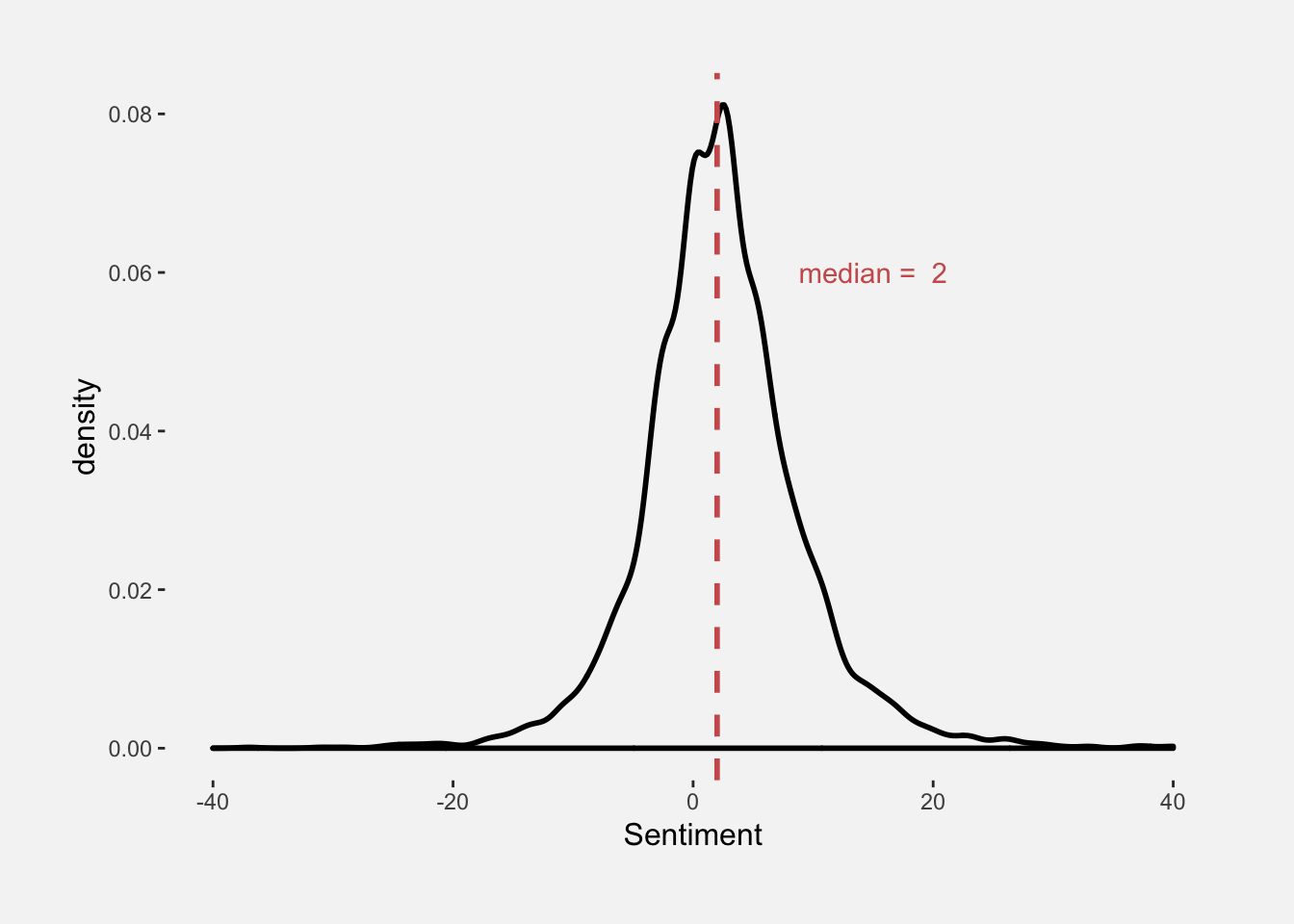
Topic modelling for positive reviews
The data frame created below contains 2228 positive reviews with scores above 1. Words will be tokenized, i.e. one word per row.
df_pos <- df            %>%
  filter(Sentiment > 1) %>%
  select(-Sentiment)    %>%
  unnest_tokens(word, Review)
Before creating a so-called document term matrix, we need to count the frequency of each word per document (review).
words_pos <- df_pos              %>%
  count(Name, word, sort = TRUE) %>%
  ungroup()

reviewDTM_pos <- words_pos       %>%
  cast_dtm(Name, word, n)
Now that we have a “DTM”, we can pass it to the LDA function, which implements the Latent Dirichlet Allocation algorithm. It assumes that every document is a mixture of topics, and every topic is a mixture of words. The k argument is used to specify the desired amount of topics that we want in our model. Let’s create a four-topic model!
reviewLDA_pos <- LDA(reviewDTM_pos, k = 4, control = list(seed = 347))The following figure shows how many reviews that are assigned to each topic.
tibble(topics(reviewLDA_pos))       %>%
  group_by(`topics(reviewLDA_pos)`) %>%
  count()                           %>%
  kable()                           %>%
kable_styling(full_width = F, position = "left")| topics(reviewLDA_pos) | n |
|---|---|
| 1 | 327 |
| 2 | 1117 |
| 3 | 266 |
| 4 | 343 |
We can also get the per-topic per-word probabilities, or “beta”.
topics_pos <- tidy(reviewLDA_pos, matrix = "beta")
topics_pos## # A tibble: 46,844 x 3
## topic term beta
## <int> <chr> <dbl>
## 1 1 telefon 0.00376
## 2 2 telefon 0.00358
## 3 3 telefon 0.0165
## 4 4 telefon 0.00319
## 5 1 abonnement 0.00326
## 6 2 abonnement 0.00871
## 7 3 abonnement 0.00193
## 8 4 abonnement 0.0130
## 9 1 navn 0.000964
## 10 2 navn 0.0000227
## # ... with 46,834 more rowsNow, we can find the top terms for each topic, i.e. the words with the highest probability/beta. Here, we choose the top five words, which we will show in a plot.
topTerms_pos <- topics_pos %>%
  group_by(topic)          %>%
  top_n(5, beta)           %>%
  ungroup()                %>%
  arrange(topic, -beta)    %>%
  mutate(order = rev(row_number())) # necessary for ordering words properly
Topic modelling for negative reviews
Let’s first do the same for negative reviews creating a data frame with 973 reviews with a sentiment score below -1.
df_neg <- df                        %>%
  filter(Sentiment < -1)            %>%
  select(-Sentiment)                %>%
  unnest_tokens(word, Review)

words_neg <- df_neg                 %>%
  count(Name, word, sort = TRUE)    %>%
  ungroup()

reviewDTM_neg <- words_neg          %>%
  cast_dtm(Name, word, n)

reviewLDA_neg <- LDA(reviewDTM_neg, k = 4, control = list(seed = 347))

tibble(topics(reviewLDA_neg))       %>%
  group_by(`topics(reviewLDA_neg)`) %>%
  count()                           %>%
  kable()                           %>%
kable_styling(full_width = F, position = "left")| topics(reviewLDA_neg) | n |
|---|---|
| 1 | 157 |
| 2 | 180 |
| 3 | 349 |
| 4 | 231 |
topics_neg <- tidy(reviewLDA_neg, matrix = "beta")

topTerms_neg <- topics_neg          %>%
  group_by(topic)                   %>%
  top_n(5, beta)                    %>%
  ungroup()                         %>%
  arrange(topic, -beta)             %>%
  mutate(order = rev(row_number())) # necessary for ordering words
Plotting the topic models
Finally, let’s plot the results…
plot_pos <- topTerms_pos %>%
  ggplot(aes(order, beta)) +
  ggtitle("Positive review topics") +
  geom_col(show.legend = FALSE, fill = "steelblue") +
  scale_x_continuous(
    breaks = topTerms_pos$order,
    labels = topTerms_pos$term,
    expand = c(0,0)) +
  facet_wrap(~ topic,scales = "free") +
  coord_flip(ylim = c(0,0.02)) +
  my_theme() +
  theme(axis.title = element_blank())

plot_neg <- topTerms_neg %>%
  ggplot(aes(order, beta, fill = factor(topic))) +
  ggtitle("Negative review topics") +
  geom_col(show.legend = FALSE, fill = "indianred") +
  scale_x_continuous(
    breaks = topTerms_neg$order,
    labels = topTerms_neg$term,
    expand = c(0,0))+
  facet_wrap(~ topic,scales = "free") +
  coord_flip(ylim = c(0,0.02)) +
  my_theme() +
  theme(axis.title = element_blank())

grid.arrange(plot_pos, plot_neg, ncol = 1)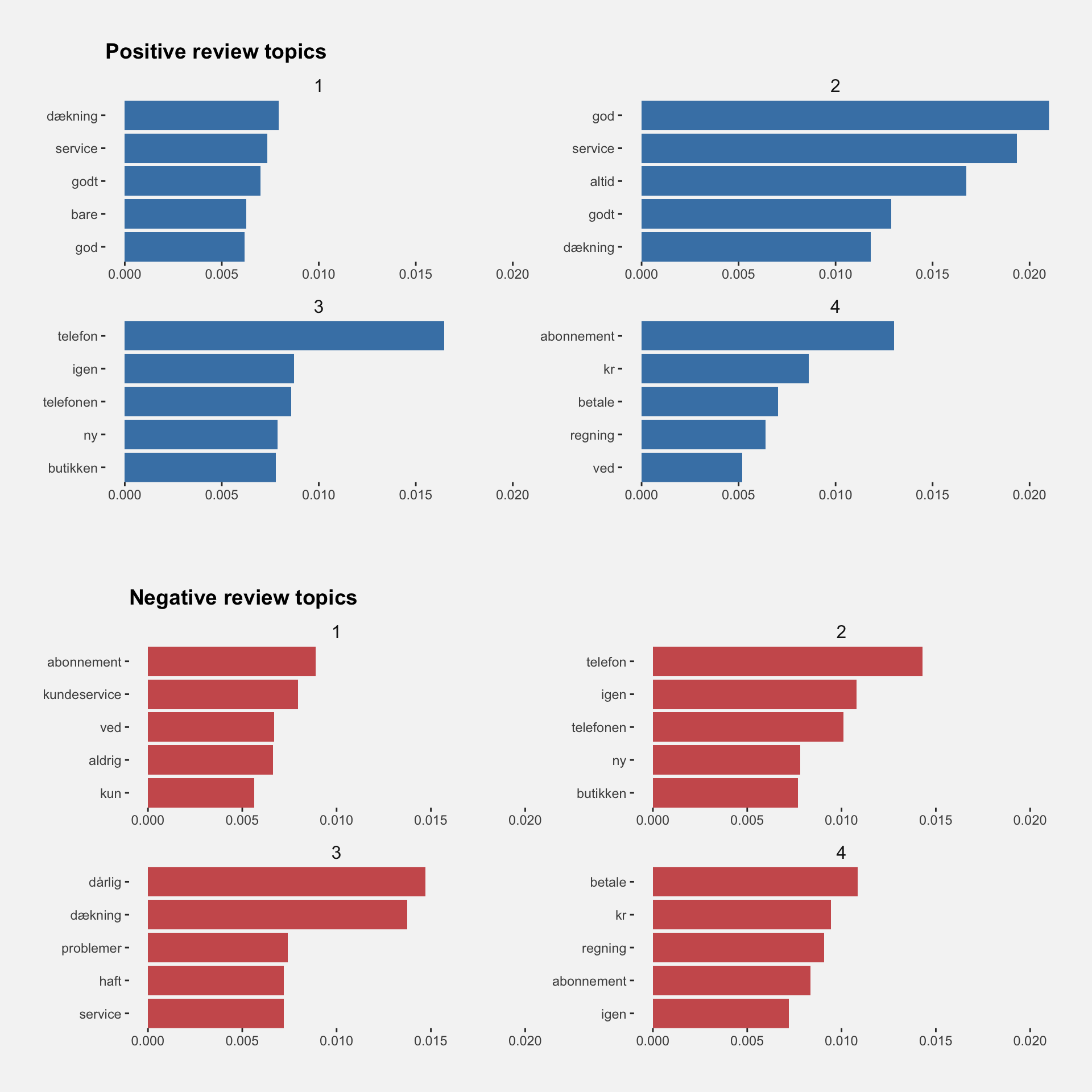
So, what do 3 customers writing reviews on Trustpilot.dk like and dislike? Unfortunately, the reviews are in Danish, but here’s what people tend to highlight, given four-topic models of positive and negative reviews:
Positive Reviews:
- coverage and data
- service
- phone, again, store and new - maybe 3 stores often replace malfunctioning cell phones?
- plan (service), kr (Danish currency), pay, bill - something positive about plans and payment?
Negative reviews:
- customer service, plan
- customer service, phone, error, plan
- phone, coverage, store
- pay, bill, kr, plan
Interestingly, customers seem to have both positive and negative experiences with respect to pretty much the same topics. Some customers appear to experience good coverage, whereas others seem to complain about poor coverage. The same pattern appears for (customer) service and payment.
Let’s explore this further..
Word co-occurrence within reviews
To see whether word pairs like “good service” and “bad service” are frequent in our two data sets, we’ll count how many times each pair of words occurs together in a title or description field. This is easy with pairwise_count() from the widyr package.
word_pairs_pos <- df_pos %>%
  pairwise_count(word, Name, sort = TRUE)

word_pairs_neg <- df_neg %>%
  pairwise_count(word, Name, sort = TRUE)
We can then plot the most common word pairs co-occurring in the reviews by means of the igraph and ggraph packages.
set.seed(611)

pairs_plot_pos <- word_pairs_pos %>%
  filter(n >= 140)               %>%
  graph_from_data_frame()        %>%
  ggraph(layout = "fr") +
  geom_edge_link(aes(edge_alpha = n, edge_width = n), edge_colour = "steelblue") +
  ggtitle("Positive word pairs") +
  geom_node_point(size = 5) +
  geom_node_text(aes(label = name), repel = TRUE,
                point.padding = unit(0.2, "lines")) +
  my_theme() +
  theme(axis.title = element_blank(),
      axis.text = element_blank(),
      axis.ticks = element_blank())

pairs_plot_neg <- word_pairs_neg %>%
  filter(n >= 80)                %>%
  graph_from_data_frame()        %>%
  ggraph(layout = "fr") +
  geom_edge_link(aes(edge_alpha = n, edge_width = n), edge_colour = "indianred") +
  ggtitle("Negative word pairs") +
  geom_node_point(size = 5) +
  geom_node_text(aes(label = name), repel = TRUE,
                 point.padding = unit(0.2, "lines")) +
  my_theme() +
  theme(axis.title = element_blank(),
        axis.text = element_blank(),
        axis.ticks = element_blank())

grid.arrange(pairs_plot_pos, pairs_plot_neg, ncol = 2)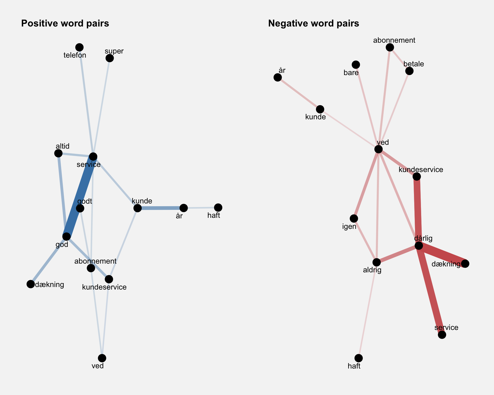
In the positive reviews, it is clear that the word for “good” (“god”) tends to co-occur with the word for “service”, “coverage” and “always”. In the negative reviews, we see that “bad” (“dårlig”) co-occurs with “service”, “coverage” and “never”. The pattern is very much the same, yet opposite!
Word pair correlations
A more direct approach to finding out what customers consider good and bad about 3 is to use the pairwise_cor() function and look specifically for the words that correlate the most with the words for “good” and “bad” in Danish. Alternatively, we could perform an n-gram analysis to find out which words most frequently follow “good” and “bad”.
cor_pos <- df_pos                       %>%
  group_by(word)                        %>%
  filter(n() >= 100)                    %>%
  pairwise_cor(word, Name, sort = TRUE) %>%
  filter(item1 == "god")                %>%
  top_n(7)

cor_neg <- df_neg                       %>%
  group_by(word)                        %>%
  filter(n() >= 100)                    %>%
  pairwise_cor(word, Name, sort = TRUE) %>%
  filter(item1 == "dårlig")             %>%
  top_n(7)
Let’s combine the data in a single plot.
cor_words <- rbind(cor_pos, cor_neg) %>%
    mutate(order = rev(row_number()),
           item1 = factor(item1, levels = c("god", "dårlig")))

cor_words %>%
  ggplot(aes(x = order, y = correlation, fill = item1)) +
  geom_col(show.legend = FALSE) +
  scale_x_continuous(
    breaks = cor_words$order,
    labels = cor_words$item2,
    expand = c(0,0)) +
  facet_wrap(~item1, scales = "free") +
  scale_fill_manual(values = c("steelblue", "indianred")) +
  coord_flip() +
  labs(x = "words") +
  my_theme()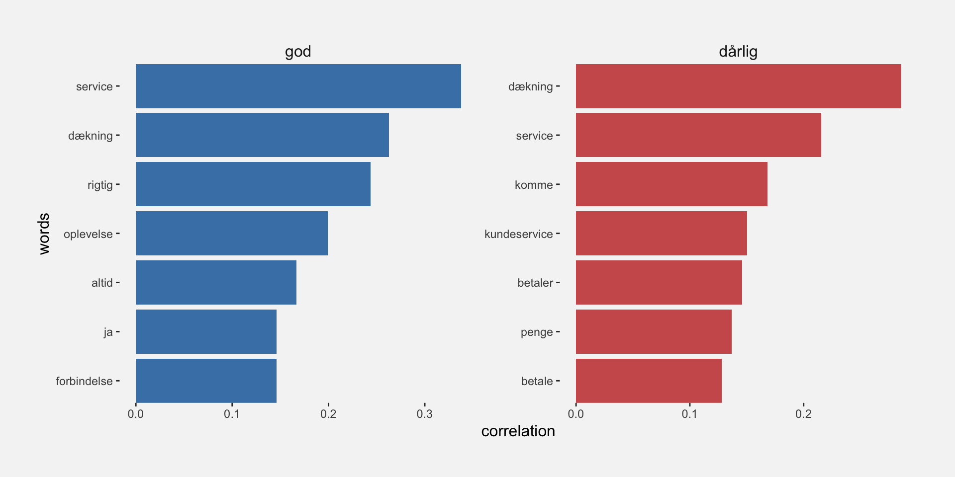
This analysis confirms that some reviewers like the (customer) service and the coverage provided by 3, whereas others have a negative view of their service and coverage.